Comprehensive model of real flushing systems - Part 2 -

The model presented can be used to calculate rinsing cascades, whereby immersion and spray rinsing can also be represented for non-ideal rinsing. The flexible model can also be used to calculate circuit flushing, recirculation flushing and spray chamber flushing.

3 Extended flushing model

The steady-state model equations previously published in [12] and [13] and summarized again in Section 2 cover a wide range of practically relevant flushing structures and effects. In order to open up further relevant applications, two structural extensions will now be introduced.

3.1 Flexible water supply

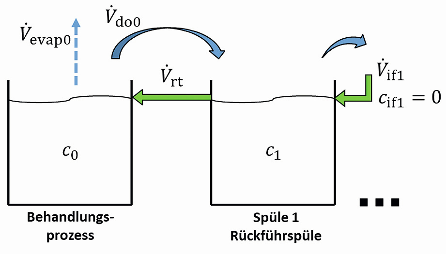
In the flushing cascade shown in Figure 2, the flushing water is fed exclusively into the last flushing stage. This makes sense and is the most frequently used form of feed. Nevertheless, in practice there are also cascade flushing systems where, for various reasons, the water is fed into the front flushing stages. If this is to be modeled, the equations <6> are extended by feeds (V_.if1, V_.if2, ..., V_.if,n-1) into the front stages:

<19>

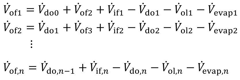
The mass flow equations <7> are extended accordingly for the case that the inlet volume flows contain the substance under consideration with the concentrations(_cif1, _cif2, ..., cif_,n-1):

<20>

3.2 Spray rinsing with fresh water

Fig. 6: Spray rinsing cascade - spraying with fresh water over all stages

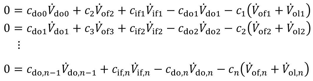
In the model presented so far, the case of spray rinsing in the cascade was shown in which spraying with rinsing water from the following rinsing stage takes place above a rinsing stage. In practice, however, external water is often also sprayed in the front rinsing stages. A corresponding cascade structure is shown in Figure 6 . Equations <18> are modified to model this structure:

<21>

If spraying is also carried out above the treatment process, the same applies:

<22>

Here csr_,k is the spray rinse concentration of the external spray solution. In most practical cases, spraying is carried out with fresh water. Then the corresponding concentration _csr = 0 and the equation <17> is simplified:

<23>

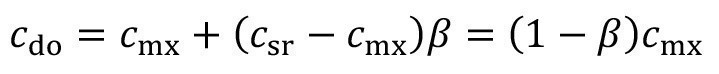
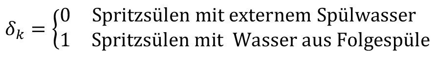
To represent the two forms of spray rinsing shown in equations <18> and <21> and <22> compactly in a model, the structural parameter _δk is introduced:

<24>

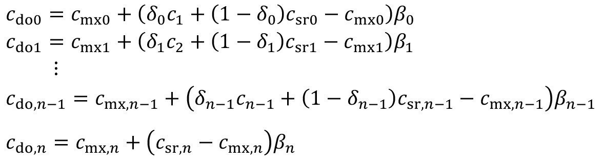
Here means:

<25>

To take the external spray rinsing volume flows (V_.sr1, V_.sr2, ..., V_.sr,n-1) into account, the volume flow equations <8> and <19> must be extended accordingly:

<26>

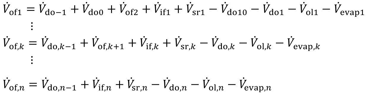
The mass flow equations <9> and <20> must be extended accordingly to include the possible entries due to spray flushing:

<27>

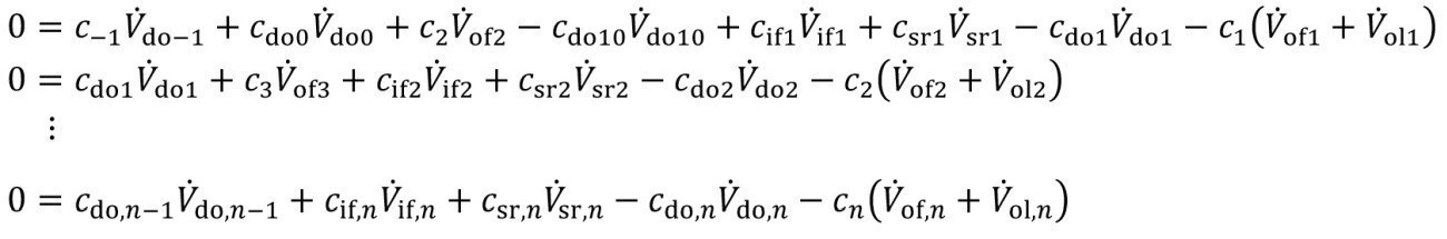
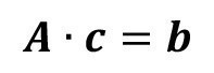
3.3 Overall model

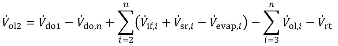
The mass flow equations <27> represent a linear system of equations. As already introduced in [12] and [13], the extended flushing model should also be expressed as a matrix equation of the form

<28>

should also be represented.

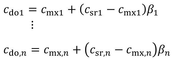
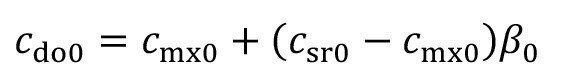
The extended matrix model results from the equations of incomplete mixing <11> and <15> as well as from the spray flushing equations <24>. The expanded volume flow and coefficient matrix A then looks as follows

<29>

The volume flows in the upper part of the matrix are calculated according to equations <26>.

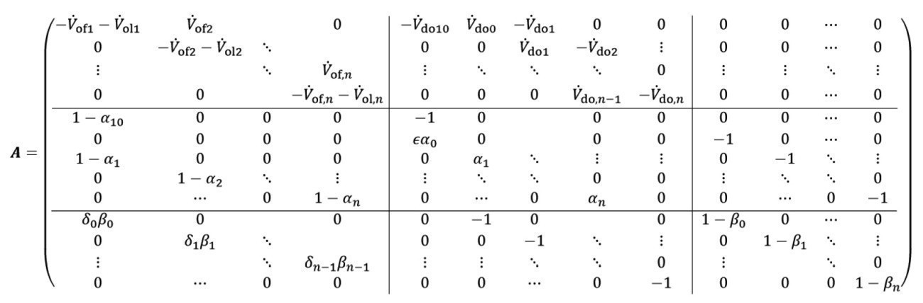
The concentration vector c used in equation <28> is made up of the concentrations in the rinsing stages _ct, the drag-out concentrations _cdo and the concentrations after removal of the product_cmx:

<30>

On the right-hand side of the matrix equation <28> is the extended entry vector b, which has the generalized form

<31>

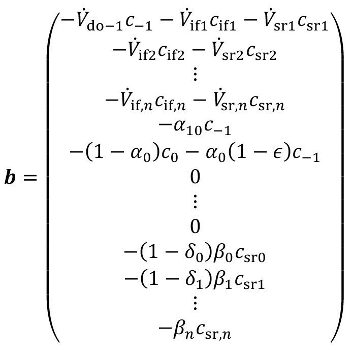
The input vector is often simplified if the additional water fed in and the spray rinse water are fresh water, i.e. the corresponding zero concentrations are _csr= 0 and _cif= 0:

<32>

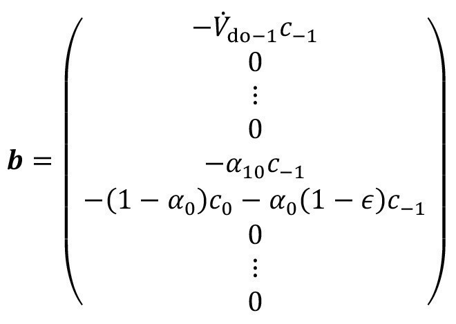
The input vector b is even simpler if, as in most practical cases, the rinse upstream of the process does not contain the substance under consideration(_c-1 = 0) and ideal mixing prevails in the treatment process due to the corresponding residence time (_α0 = 0). Then the entire input vector b is only occupied at the(n+2)th position with the process concentration _-c0; all other elements of the vector have the value zero.

4 Use of the model 4.1 Calculation of flushing concentrations

If all the necessary parameters are known for a given flushing system structure, the stationary flushing concentrations can be calculated using the flushing model presented. To do this, the linear system of equations shown in equations <28> to <32> must be solved. In matrix form, the concentration vector sought is calculated with

<33>

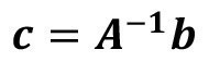
This means that the inverse of the volume flow and coefficient matrix b is multiplied by the entry vector A on the right-hand side.

The following steps are therefore necessary to calculate the flushing concentrations:

1. collation of all relevant model parameters

• Carryover volume flows
• Inlet volume flows
• Concentration in the treatment process
• Factors of incomplete mixing
• Discharge volume flows, if applicable
• Pre-immersion, if applicable (structural parameters for case differentiation) and, if applicable, concentration of the upstream sink
• Evaporation from rinsing stages, if applicable
• Spray rinsing, if applicable

- Spray rinsing factors
- Spray rinsing volume flows
- Structural parameters for the source of the spray rinse
(secondary rinse or fresh water)

• If applicable, concentration of supplied volume flows (supply, external spray rinse water)

2. calculation of the overflow volume flows (equations <26>)

3. formulation of the matrix model by setting up

• the volume flow and coefficient matrix A (equation <29>)
• of the input vector b (equation <30>)

4. calculation of the inverse of the volume flow and coefficient matrix ^A-1

5. calculation of the required concentration vector c by matrix multiplication (equation <33>)

4.2 Calculation of the water requirement

The calculation of the concentrations for a given operating scenario shown in section 4.1 represents a direct solution to the problem for a given flushing system. In practice, however, the question is often the other way round. What is required is the rinsing quality to be achieved by the product after passing through the cascade rinse. A rinsing criterion is specified here, which indicates how the dilution of the drag-out remaining on the product should be in relation to the concentration in the treatment process:

<34>

The required rinsing water volume flow must therefore be determined for a specified carryover concentration. The corresponding flushing problem must therefore be solved indirectly.

An explicit solution to this indirect problem cannot be formulated in a generally valid way. However, it is possible to solve the indirect problem by repeatedly calculating the model equation <33> with different flushing volume flows. The required volume flow is changed until the required carryover concentration is obtained. Mathematically, this procedure corresponds to solving an optimization problem. The simplest case is when only the feed volume flow into the last sink is changed in order to achieve a specified carryover concentration from the last sink. This one-dimensional optimization problem can be solved using simple tools (e.g. target value search in Microsoft Excel) or even by trial and error.

The solution to the indirect problem becomes more complicated if several volume flows are to be modified. This is the case, for example, with the spray rinsing with fresh water shown in Figure 6. Here, the spray rinsing volume flows V_.sr,k can be modified over the various rinsing stages in order to adjust the concentration ratios in the rinsing cascade.

In this way, a number of spray rinsing volume flows can also be used to set a corresponding number of n concentrations in the rinsing system. If n concentrations are specified and n corresponding volume flows are sought, an n-dimensional optimization problem must be solved. The corresponding mathematical optimization can be carried out using suitable computer tools. For the MATLAB mathematical software, for example, there is an optimization toolbox that provides various powerful algorithms for multidimensional optimization. For Excel, on the other hand, multidimensional optimization problems can be solved with the Solver add-in.
optimization problems can be solved with the solver add-in. The two tools mentioned also allow searching with constraints. This is helpful to exclude technically unfeasible cases (e.g. negative volume flows) or to only allow certain value ranges for searched variables.

5 Calculation of special design variants

In Section 3, the stationary flushing cascade model was structurally extended compared to previously published versions in order to represent a wider range of practically relevant flushing system variants. This section will now show how special design variants of flushing systems can be mapped by selecting suitable parameters.

5.1 Circulation rinsing

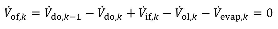
A simplified model approach is sufficient to illustrate the corresponding processes. Figure 7 shows the corresponding diagram. It is assumed that the volume flows at the inlet and outlet of the ion exchanger are the same:

<35>

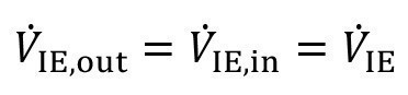
As long as the ion exchangers are operated without breakthrough, it can be assumed that the ions are completely removed. This means that the corresponding substance can no longer be found at the outlet of the ion exchanger:

<36>

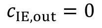
Accordingly, there is a mass flow of a dissolved substance flowing into the ion exchanger

<37>

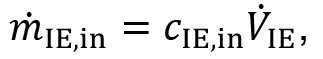
whereas the mass flow at the outlet is zero:

<38>

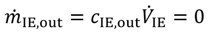
This very simple model is included in the general flushing model when illustrating an ion exchange circuit. When the ion exchanger is connected to the kth rinsing stage, the outlet and inlet of this stage are set equal to the circuit volume flow:

<39>

<40>

With complete depletion, the concentration of the water flowing back from the ion exchanger into the recirculation sink is as follows

<41>

The rinsing stage, which serves as a recirculation rinse, is usually operated separately. This means that there is no overflow volume flow that flows into the upstream rinsing stage. With the same inlet and outlet in the circuit according to equations <39> and <40>, the same drag-in and drag-out and negligible evaporation, the following applies:

<42>

In most cases, the recirculation sink is implemented as a final sink. A corresponding diagram is shown in Figure 8. In the above equations, the number of stage k must be replaced by n accordingly.

Fig. 8: Rinsing cascade with ion exchange circuit rinse

To take the ion exchange circuit into account in the rinsing cascade model introduced in section 3, the parameters for the associated rinsing stage must be assigned in accordance with equations <39> to <41>. In addition, the conditions specified for the validity of equation <42> must be fulfilled. Then the special case of recirculation flushing can also be calculated using the general stationary flushing cascade model. A calculation example of a cascade flush with a final recirculation flush follows in section 6.2.

5.2 Recirculation sink

A design variant frequently used in practice is the operation of the first rinsing stage as a recirculation sink (also known as an "economy sink"). In this case, a certain volume flow is returned to the treatment process from the first, still relatively highly concentrated rinse. This return volume flow transports valuable substances (metal ions, process chemicals). In this way, some of the valuable substances discharged from the treatment process as a result of carryover can be recovered and do not enter the wastewater treatment and are therefore lost to the process.

The recirculation sink is usually operated as a so-called "stationary sink". This means that the cascade counterflow is not fed from the second rinse into the first stage. The first rinsing stage is therefore no longer part of the flow cascade. However, "stationary sink" here does not mean that there is no "flow" at all - i.e. no inflow and outflow - in the recirculation sink. On the contrary, a small volume flow from the recirculation sink is fed back into the treatment process; it is precisely this volume flow that realizes the desired material recirculation. The recirculation volume flow is generally selected according to the evaporation in the treatment process:

<43>

Filling with fresh water

In order to be able to model the filling of the recirculation sink with fresh water (Fig. 9), the first sink is mentally removed from the counterflow cascade. This means that the overflow volume flow from stage 2 must be zero. For this purpose, the outflow volume flow from stage 2 is selected to be equal to the sum of the inflows and outflows in stage 2:

<44>

Fig. 10: Recirculation sink with supply from the next stage

If the overflow volume flow is now replaced in this equation and successively in the following equations with the volume flow equations <26>, the result for the overflow-free second sink is

<45>

It should be noted that the spray rinsing volume flows V_.sr,i listed in equation <45> only apply to spraying with (external) fresh water, see section 3.2. If spraying is carried out with water from the following rinsing stage, the corresponding terms V_.sr,i do not apply. Filling the recirculation rinse with fresh water takes place according to the recirculation:

<46>

If there is a relevant difference between drag-in and drag-out or evaporation in the recirculation sink, this must also be taken into account in the volume flow V_.if1 . If the possible recirculation volume flow is relatively high, the volume deficit in the recirculation sink can also be compensated by spray rinsing instead of inflow.

Filling from the next stage

To model the filling of the recirculation sink with rinse water from the second rinsing stage (Fig. 10), the equation <45> is changed so that the remaining overflow from stage 2 into the recirculation sink corresponds to the recirculation volume flow _Vrt:

<47>

An external feed flow into the recirculation sink is then no longer necessary:

<48>

Discontinuous recirculation

The recirculation process considered up to this point is described as a continuous process. This means that recirculation is always realized by a constant, continuous volume flow V_.rt. The same applies to the compensation of the deficit in the recirculation sink. In practice, this is a frequently used operating regime in which the treatment process continuously "draws" the rinsing water required for replenishment from the recirculation sink according to the evaporation via a fill level control.

A variant that is also regularly used is discontinuous recirculation. In this case, the return from the first rinse to the treatment process only takes place at certain intervals. With the corresponding discontinuous mode of operation, there are fluctuations in volume and concentration in the treatment process and in the sinks. In principle, these fluctuations cannot be mapped in the stationary model introduced here, as it has just been assumed for the stationary state according to equations <2> and <5> that the tank volume and concentrations are in equilibrium and no longer change. In individual cases, it can be checked whether the steady-state model can still be used to calculate approximate solutions with only small fluctuations.

5.3 Spray chamber purging

Fig. 11: Spray chamber purging

The spray rinsing described in sections 2.3 and 3.2 is, strictly speaking, a combined immersion and spray rinsing. As Figure 4 illustrates, the fabric is first immersed in a rinsing tank filled with rinsing water. Then the goods are additionally rinsed by spraying when they are removed.

In contrast to this, spray chamber rinsing is also used in practice. Here, the fabric is sprayed in an empty container(Fig. 11). Spraying takes place when the fabric is moved in and out. Sometimes there is also a certain idle time during which water is also sprayed off.

The spray chamber rinse can also be represented with the general stationary rinsing model presented here. The missing filling volume for spray chamber rinsing is not a problem for the application of the model, as the volume is not shown in the stationary model. Compared to combined immersion/spray rinsing, immersion rinsing is not required for spray chamber rinsing. This can be represented in the stationary model by setting the incomplete mixing factor to one. Immersion rinsing is then completely ineffective; it therefore does not exist:

<49>

The effect of spray chamber rinsing is again represented by the spray rinsing factor _ßk according to equation <17>. However, it can be assumed that the spray rinsing factors are higher for spray chamber rinsing than for combined immersion spray rinsing. This is due in particular to the fact that a larger quantity of spray water is generally used for spray chamber rinsing than for spraying over an immersion rinse. In addition, when spraying inside the spray chamber, a greater intensity (pressure and volume flow) can be used.

Literature

[12]Giebler, E.: A General Steady State Model of Cascade
Rinsing Systems, Transactions of the Institute of Metal
Finishing 82 (2004) 3/4, 75-82
[13]Giebler, E.; Röbenack, K.: Flexible Design Calculations for Rinsing Cascades - Part 1/2, Galvanotechnik 98 (2007) 2/3, 474-480 / 753-759
[16]Dietrich, G.: Hartinger - Handbuch Abwasser- und
Recyclingtechnik, 3rd edition, Carl Hanser Verlag, Munich, Vienna, 2017