
The second series of measurements / continued from issue 11/21
Comparison of the two-dimensional roughness values with the surface roughness values
With this knowledge and the realization that the optical measuring devices guarantee absolutely comparable measured value acquisition, the 2D and 3D measured values can now be compared (Fig. 16 and 17).
 und 17 (rechts): Vergleich verschiedener Rauheitswerte aus taktilen und optischen, zweidimensionalen Messungen mit Flächenwerten für das Drehteil (links) und das gefräste Teil (rechts)") Fig. 16 (left) and 17 (right): Comparison of different roughness values from tactile and optical, two-dimensional measurements with surface values for the turned part (left) and the milled part (right)
Fig. 16 (left) and 17 (right): Comparison of different roughness values from tactile and optical, two-dimensional measurements with surface values for the turned part (left) and the milled part (right)
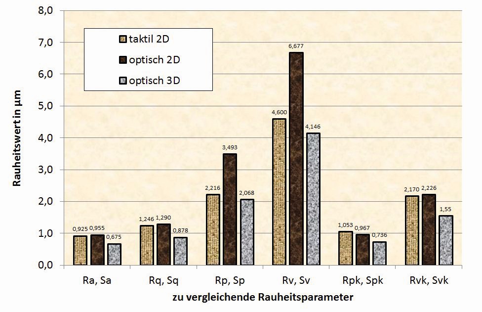
When comparing the values forRa and Rq withSa and Sq, it can be seen that the values hardly differ and are therefore comparable for both the line and the surface. This is due to the fact that all measured points of the line or surface under consideration are used for averaging, i.e. not only individual elevations or depressions, but all measured points, including those near the center line or the average surface between the enveloping elevations and depressions. Therefore, the values are also very low compared to the extreme values and are not very meaningful with regard to the actual appearance or behavior of the surfaces. The fact that the area values are slightly lower than the line values is due to the larger number of measured values, because if the detection of an area can be approximated as a grid of adjacent lines, it is conceivable that there are other points between the lines near the center, which are also included for averaging and thus lower the mean value somewhat further.
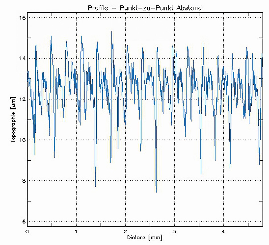
This is very different when comparing Rp or Rv withSp orSv and also when comparing the turned surface with the milled surface. While the differences between the tactile and visually measured line values can be explained by the behavior of the values for Rz (shown visually in Figs. 12 and 14 ), the surface valuesSp andSv are clearly too high for the turned surface. Although the line values are mean values from 10 measurements, there are areas between these 10 lines that are not recorded in the two-dimensional measurement and it can be assumed that there are elevations or depressions that are recorded in the area measurement and thus increase the measured value. To discuss the lower values forSp andSv for the milled surface, the profiles of the two surfaces must be used (Fig. 18 and 19) to come closer to an explanation. The turned surface is less rough overall than the milled surface and has significantly less pronounced elevations or depressions. Most of the measured values for the turned surface are therefore relatively close together or more close to the center line, resulting in a flat Abott curve and large values forSp andSv. The few pronounced peaks and troughs are "cut off" relatively far. With the milled surface, there are many more pronounced peaks and valleys in accordance with the machine's feed rate, resulting in a rather steep Sp curve and therefore the values forSp andSv are comparatively small. This difference has a more pronounced effect on the surface than when only one line is measured.
 und 19 (rechts): Vergleich der Profilschnitte aus der optischen, zweidimensionalen Messung der Linie 1 für das Drehteil (links) und das gefräste Teil (rechts)") Fig. 18 (left) and 19 (right): Comparison of the profile sections from the optical, two-dimensional measurement of line 1 for the turned part (left) and the milled part (right)
Fig. 18 (left) and 19 (right): Comparison of the profile sections from the optical, two-dimensional measurement of line 1 for the turned part (left) and the milled part (right)
For the values according to DIN EN ISO 13565, the trend is similar to that just described, with the exception of the valueSvk for the turned part. This is due to the fact that a few extremely deep valleys occur, which have a similar effect onSvk as on the milled part, but not onSv. It should also be noted that the figures for the load-bearing components are in a similar range when viewed generously (see Table 1).
|
Turning |
Milling |
|||||
|
Line |
Surface |
Line |
surface |
|||
|
tactile |
optical |
tactile |
optical |
|||
|
Mr1,Smr1 |
4,6 % |
8,7 % |
6,8 % |
12,1 % |
11,2 % |
10,4 % |
|
Mr2,Smr2 |
80,0 % |
84,0 % |
87,9 % |
77,9 % |
81,2 % |
78,4 % |
|
Rsk, Ssk |
-0,91 |
-0,98 |
0,20 |
-1,08 |
-1,14 |
-0,88 |
The smaller values forMr1 andSmr1, but also forMr2 andSmr2 for turning compared to those for milling are consistent with the statements on the slope of the Abott curve.
The comparison of the skewness Rsk or Ssk with the predominantly negative values essentially indicates that the surfaces tend to plateau, i.e. that the valleys are more prominent than the hills. This is also the case for the milled part in the areal measurement, but not for the rotated part. Here, the measurement over the surface seems to produce a different result than the measurement of a few lines, which would have to be investigated in more detail with additional measurements to obtain a very differentiated statement.
Discussion based on a second series of measurements
A workpiece as shown in Figure 1 was carefully turned flat and then sanded by hand with a sanding belt (grain size 400, SiC) in one direction until the turning grooves were no longer visible in order to obtain a smooth and uniform surface with only one direction of grooves. Figure 20 shows the image taken from above with a Keyence VR-5000 profilometer.
 Fig. 20: Flat surface of a belt-ground workpiece; image taken with Keyence VR-5000 profilometer; right in the image: test measurement
First, the measurement was again carried out with the stylus instrument (Fig. 21) with the result of a roughness of Rz = 5.8 µm and a plateau-like profile, which can be seen both in the profile itself and in the contact ratio curve as well as in the amplitude density distribution. The same applies to the values for Rp = 1.79 µm and Rv = 4.01 µm as well as Rsk = -1.305.
 und Traganteilkurve (rechts) eines bandgeschliffenen Werkstücks mit dem Tastschnittgerät gemessen") Fig. 21: Roughness profile (left) and contact ratio curve (right) of a belt-ground workpiece measured with the stylus instrument
Fig. 21: Roughness profile (left) and contact ratio curve (right) of a belt-ground workpiece measured with the stylus instrument
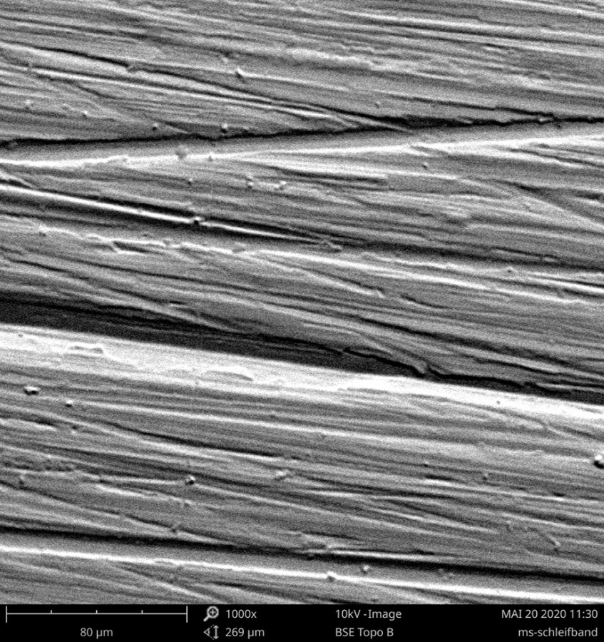
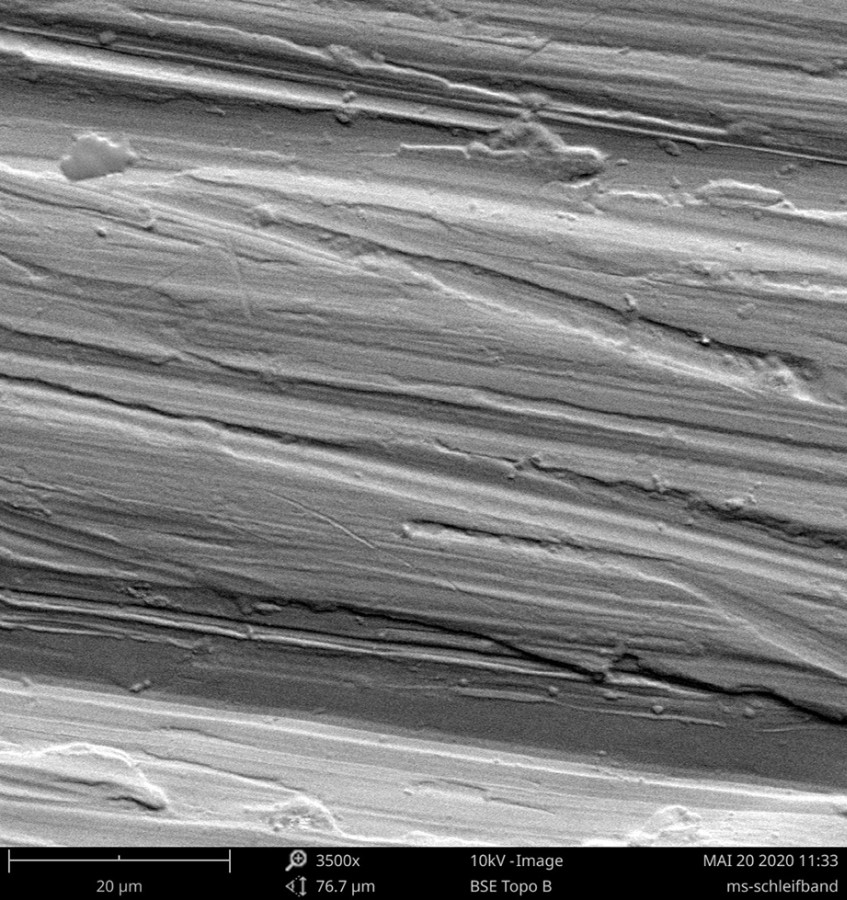
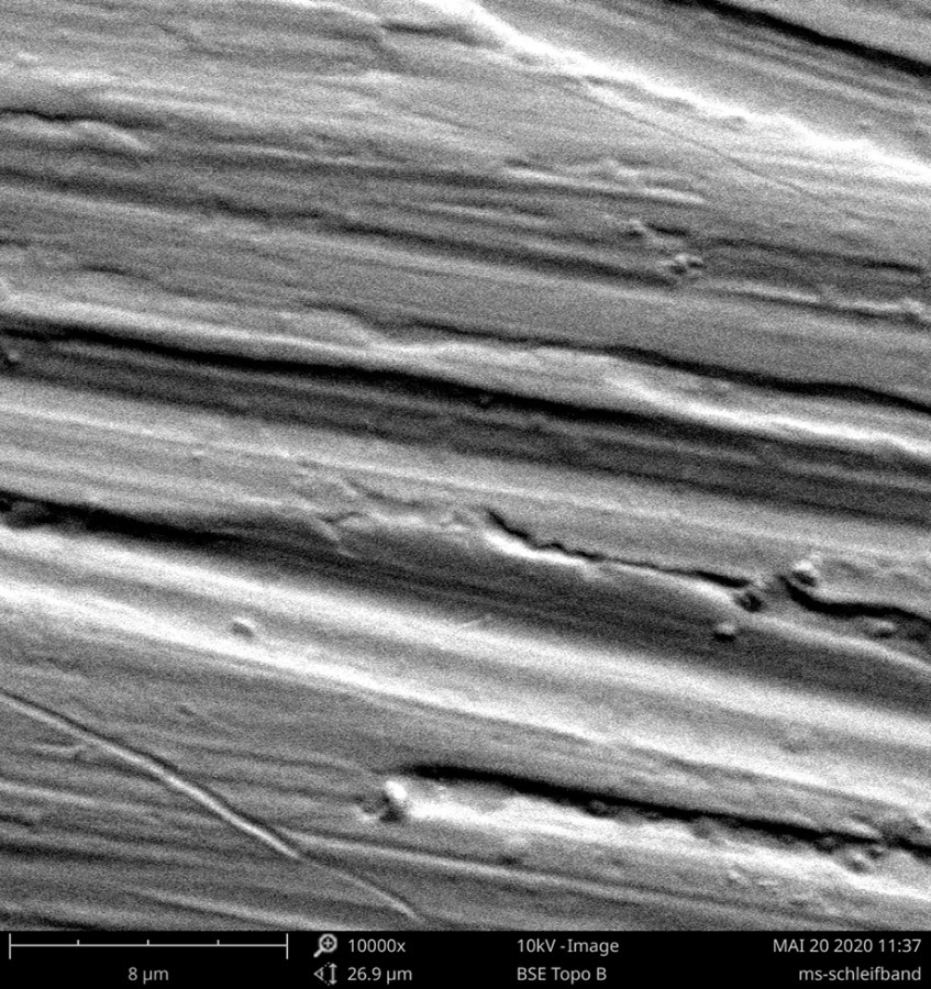
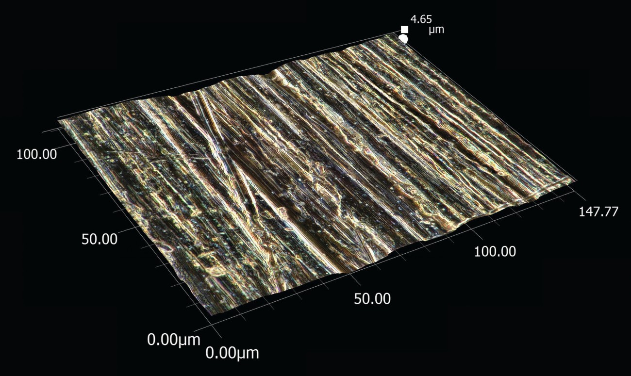
To provide a visual impression of this surface in addition to the measured values, the surface was photographed with a Keyence VHX-7000 digital microscope and a Phenom Pro X scanning electron microscope (Figs. 22 to 29). It can be seen from the images that the surface is rather smooth, with grooves and generally few elevations. It is also clear to see that the material between the individual grooves is smooth and without any further markings from the abrasive grains. The surfaces are even easier to visualize in a 3D representation (Fig. 30 to 32).

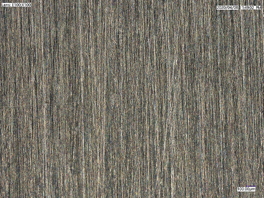
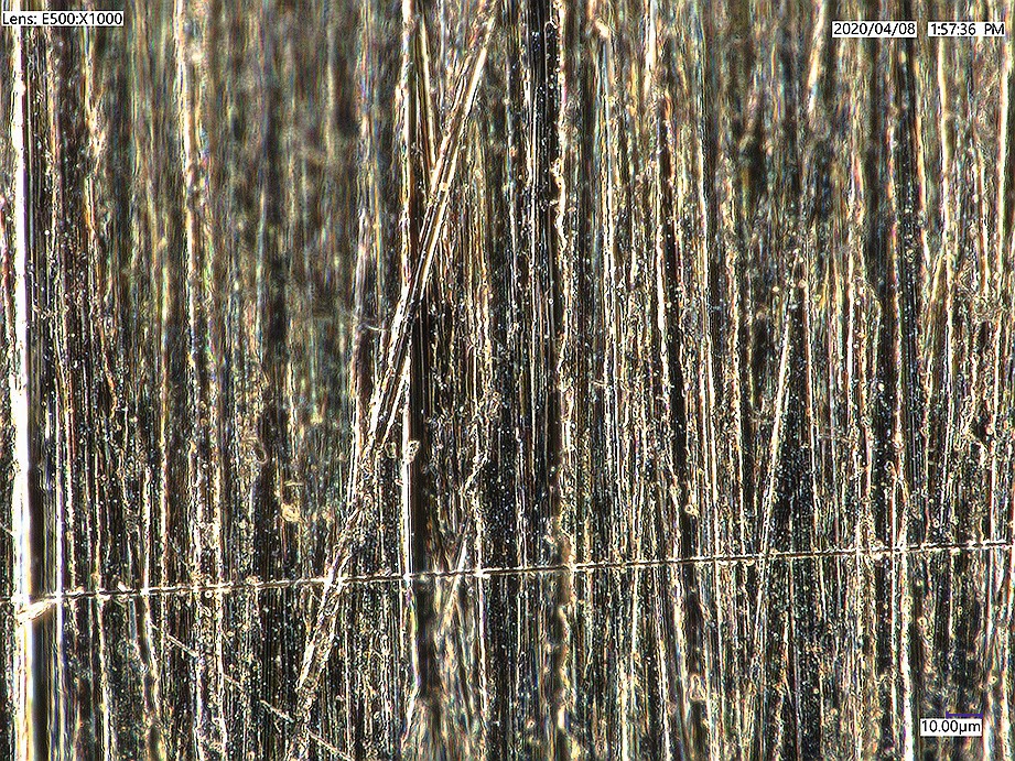
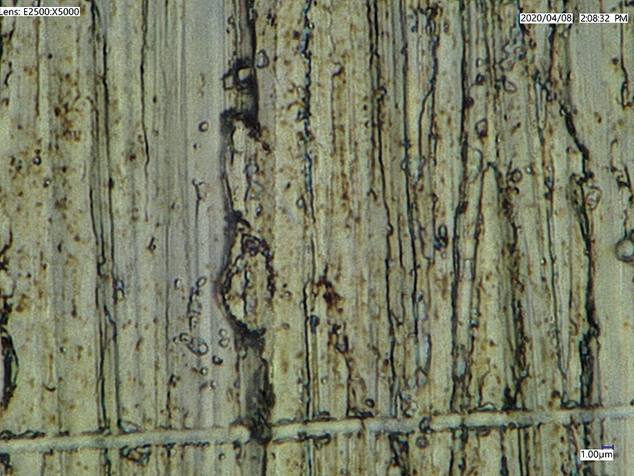
 sowie mit einem Rasterelektronenmikroskop Phenom Pro X (untere Reihe, in Vergrößerungen von 300, 1.000, 3.500 und 10.000)") Fig. 22 to 29: Images of the belt-ground surface with a Keyence VHX-7000 digital microscope (top row, magnifications of 20, 100, 1,000 and 5,000) and with a Phenom Pro X scanning electron microscope (bottom row, magnifications of 300, 1,000, 3,500 and 10,000)
Fig. 22 to 29: Images of the belt-ground surface with a Keyence VHX-7000 digital microscope (top row, magnifications of 20, 100, 1,000 and 5,000) and with a Phenom Pro X scanning electron microscope (bottom row, magnifications of 300, 1,000, 3,500 and 10,000)
Without going into further details for this series of measurements, the measured values from two 2D measurement series and two 3D measurement series are compared here in Figure 33, analogous to Figures 16 and 17.
 Fig. 30 to 32: 3D images of the belt-ground surface with a Keyence VHX-7000 digital microscope at magnifications of 500, 2,000 and 5,000; the respective heights of the profiles shown are approx. 16, 5 and 4 µm from left to right

") Fig. 33: Comparison of different roughness values from a tactile and an optical, two-dimensional measurement with area values from two measuring devices for the belt-ground surface (WLI...white light interferometer)
Fig. 33: Comparison of different roughness values from a tactile and an optical, two-dimensional measurement with area values from two measuring devices for the belt-ground surface (WLI...white light interferometer)
![Abb. 35: Drei nebeneinander liegende Profilschnitte auf einer unregelmäßigen Fläche mit abweichenden Rauheitswerten [5]](/images/stories/Abo-2021-12/gt-2021-12-0072.jpg "Abb. 35: Drei nebeneinander liegende Profilschnitte auf einer unregelmäßigen Fläche mit abweichenden Rauheitswerten [5]") Fig. 35: Three adjacent profile sections on an irregular surface with deviating roughness values [5]
Fig. 35: Three adjacent profile sections on an irregular surface with deviating roughness values [5]
 sowie Rauheitsprofil (rechts) der 2D-Messung mit dem Weißlichtinterferometer") Fig. 34: Top view with height profile and measurement line (left in blue) and roughness profile (right) of the 2D measurement with the white light interferometer
Fig. 34: Top view with height profile and measurement line (left in blue) and roughness profile (right) of the 2D measurement with the white light interferometer
|
2D |
3D |
|||
|
Tactile |
White light |
white light |
profilometer |
|
|
Mr1,Smr1 |
4,6 % |
9,2 % |
7,1 % |
9,9 % |
|
Mr2,Smr2 |
83,3 % |
87,5 % |
88,0 % |
88,7 % |
|
Rsk, Ssk |
-1,31 |
-1,01 |
-0,46 |
-0,12 |
The statements made for Figures 16 and 17 can be fully confirmed for this second series of measurements. All values, which are based on averaging over all points in the z-direction, are comparable both for the 2D measured values and for the 3D measured values and fluctuate within the measurement accuracy. A comparable similarity, albeit not as close, applies to the values Rk orSk, Rpk orSpk and Rvk orSvk derived from the bearing component curve in accordance with DIN EN ISO 13565. The deviations in this case are also due to the different measuring ranges because, for example, only a smaller area was selected for this measurement with the white light interferometer due to the long measuring times. The situation is different with the values for Rp orSp and Rv orSv. While individual values also behave similarly here, this is not the case at all with the value for Rp measured with the white light interferometer, for example. One possible explanation would be singular irregularities in the measurement. For example, Figure 34 shows a deep notch at x ≈ 0.2 mm and a peak close to it at x ≈ 0.3 mm, which are averaged out for values such as Ra or Sa, but clearly influence the figure for parameters that take the maximum values into account. As with the comparison of the turned and milled surfaces in measurement series 1, the other roughness parameters can also be compared in tabular form (Table 2). The fact that there are deviations in both the measured values in Figure 33 and in Table 2 can be easily explained with an example in Figure 35. Three 2D profile sections are placed next to each other in a real, albeit sometimes very irregular surface, with grooves of different depths at several points. Even with such closely spaced lines, there are deviations that lie within the range of the fluctuations that occur in our own measurement series, although care was taken to measure reasonably homogeneous areas.
- to be continued -
Literature
[1] E DIN EN ISO 25178-2: Geometric product specification (GPS) - Surface finish: Planar - Part 2: Terms, definitions and surface characteristics, Beuth-Verlag, Berlin, 2020
[2] Wiehr, C.: User support for the use and verification of optical 3D surface measuring devices. Dissertation, Technical University of Kaiserslautern, 2019
[3] Ströer, F.; Seewig, J.; Depiereux, F.: Roughness measurement tactile or optical? Comparable results. QZ 59(2014)5, 70-72
[4] Plein, C.: Comparative surface topography. Student research project. Cooperative State University, Lörrach, 2018
[5] Schorr, D.: Measurement of the Steinbeis Transfer Center Tribology in Application and Practice, Karlsruhe, 2018
[6] https://commons.wikimedia.org/w/index.php?curid=44998701
