Transfer Learning - Part 2 Automatic detection and classification of electronic components in X-ray images based on neural networks

As part of a graduation thesis, a system was developed with which convolutional neural networks (CNN) can be trained to reliably identify electronic components in X-ray images. The concept of transfer learning is used to train the CNNs. A procedure was designed and implemented to generate suitable training data sets. With the help of the training data sets, different network architectures for image classification and object detection could be trained and evaluated. For the transfer learning, freely available models from another domain were used. The results show that transfer learning is a suitable method to reduce the effort (time, amount of data) in creating classification and object detector models. The models created show a high degree of accuracy in classification and object detection, even with unknown data. Applications that are related to the evaluation of radiographic images of electronic assemblies can be designed more effectively thanks to the available knowledge.

Part 2 in this issue explains the concept of transfer learning and presents the study results.(See issue 10/2022 for Part 1)

As part of a graduate thesis, a system was developed with which Convolutional Neural Networks (CNN) can be trained to reliably recognize electronic components in X-ray images. The concept of transfer learning is used here. A procedure was designed to generate suitable training data sets. This made it possible to train and evaluate various network architectures for image classification and object detection. Freely available models from another domain were used for transfer learning. The results show that transfer learning is a suitable method for reducing the effort (time, data volume) involved in creating classification and object detector models. The created models show a high accuracy in classification and object detection even with unknown data. Applications related to the evaluation of radiographic images of electronic assemblies can thus be designed more effectively.

In the first part of the article (see issue 10/2022), the specifics of object recognition in X-ray images and the use of neural networks for such tasks were presented. The question of how existing results from the field of image recognition on light-optical images of objects from other application areas can be used to achieve results more quickly is addressed in the following.

Part 2 of this issue explains the concept of transfer learning and presents the results of the study.(Part 1 see issue 10/2022)

4 Transfer Learning

The image classification process using CNN can be visualized in compact form as shown in Figure 4. The model consists of the so-called backbone and the head. The backbone generates features from the input data by applying filters and creates feature maps. These are classified in the head. In a newly initialized neural network, the filters are initially very unspecific and are refined and optimized during training. However, reinitializing a CNN is very time-consuming and computationally intensive and requires a very large number of annotated data sets, i.e. several hundred images per object class. In this context, annotation means linking an image with the corresponding class label.

Fig. 4: Image classification process

The creation of a data set is generally regarded as the most complex and expensive process. However, the effort can be reduced by transferring the knowledge of a pre-trained neural network for solving a task to a new task or application. Transfer learning is basically the same as classification, whereby an already trained model is modified and further optimized.

Different modification scenarios are available for transfer learning and follow the following scheme:

1. Selection of a base network
2. Copying the first n layers (filter kernel)
3. Training the network with the target data set

The configuration of the target network (choice of base network, number of transferred or reinitialized layers) is freely configurable and is left to the user. However, the parameters mentioned depend on the size of the data set, the similarity to the source domain and the application and must usually be determined experimentally. It is generally recommended, especially for very small data sets, to replace only the last layer with a linear classifier [6].

(a) Starting point: Pre-trained network for a specific task

(b) Scenario 1: The pre-trained network architecture is completely transferred. The individual layers can be optimized during training

(c) Scenario 2: The first n layers are transferred and the last two are initialized with random values. The transferred layers can be trained, the newly initialized ones must be trained

(d) Scenario 3: The network is transferred, cut off after the third layer and two new layers are added, according to [6].

4.1 Data set

The requirements for a data set are largely determined by the purpose of the application. In this study, two applications in the field of machine vision were considered. The first is image classification and the second is object detection.

For classification, it is sufficient to provide one label per image. This can take the form of a folder structure in the file system or a file in which the file names are assigned to the object classes. For object detection, the coordinates of the rectangle representing the object boundaries must also be provided.

The amount of training data required for classification depends on the complexity of the task and the complexity of the model. In general, a linear relationship can be assumed between the number of parameters that can be optimized and the number of samples required. Different requirements apply to object detection, as during training, in addition to the classification of objects, the differentiation from the background must also be learned. Therefore, in addition to the quantity of data, quality also plays a very important role. However, this does not mean image quality in the conventional sense, but rather the diversity of the images. At best, a high-quality data set represents all possible shooting conditions and situations. For everyday objects, this means: illumination, time of day and season, weather and different contexts.

For the recognition of electronic components, this means that as many different assemblies and package types and sizes as possible are included in the creation of the data set. Data augmentation can be used to artificially expand the data set. This involves image transformations such as mirroring, distortions and the addition of image noise.

The data sets that were generated for the training and the tests are based on image data provided by two different assemblies from an industrial partner (see Table 2) and on images taken on test assemblies. To speed up the process, X-ray images of assemblies were automatically annotated with the corresponding design data. To achieve this, 2D codes were structured in the copper layer of the PCB, which are visible in the X-ray image and thus enable a clear assignment between the image section and the design data. When creating the data set, a balanced class distribution and a high degree of diversity in the images were taken into account. In this way, different data sets were generated for the training of image classifiers and object detectors.

Tab. 2: Information on assemblies of the data sets provided

Data set	Assembly 1	Assembly 2
Assembly Layers Technologies Components Most common components Special features	one-sided single layer SMT, THT 1492 objects 9 different component types 77 package / footprint variants Resistance - 37% Capacitance - 22% Diode - 17% Customer product (test assembly)	double-sided multilayer SMT, THT 783 objects 11 component types 57 package / footprint variants Resistance - 56% Capacitance - 24% Diode - 8.3% Customer product, image with longer exposure time, therefore less image noise

Six different SMD component and package types were used for our own test board. In this specific case, these include

• Chip resistor size 0603
• Chip capacitor size 0603
• Chip inductor size 0402
• TVS diode - bidirectional, package: SOD-882
• Transistor, Package: HUSON3 (QFN / SON)
• Schottky diode, package: SOT-143R

To avoid an unbalanced class distribution, 50 of each of the above component types are placed on the test board (300 components in total). In order to achieve the highest possible variation in the recordings, the components are not placed regularly on the board, but randomly. In this specific case, the board has dimensions of 80mm x 100mm. The random arrangement of the components can be seen in Figure 6 using the board file from the design system.

Fig. 6: Placement positions of the test board

Fig. 7: Aruco marks structured in copper, test board for examining different structure sizes (per pixel: 0.25 mm, 0.5 mm, 0.75 mm, 1 mm and 2 mm)To make it easier to automatically annotate the image data later, special reference marks in the form of Aruco marks were also placed manually on the PCB. This is a square structure with which a number is coded in the form of a pixel mask. This structure was later structured into the copper layer of the PCB together with the component connection pads. An example of these structures is shown in Figure 7. Aruco markers are a reference marker system that was originally developed for and is also used in the field of robot navigation and augmented reality applications. To increase the amount of data, several images are taken per board, with different structures superimposed on the test board.

For the automatic annotation of the image data, at least one of the reference marks should be present in the image, but two would be better. Another prerequisite is the provision of the CAD data associated with the board in the form of a board file. The use of Aruco markers offers several advantages for automated annotation compared to the usual reference markers in the form of circles, squares or crosses. Often only individual images of parts of an assembly are taken. Although reference marks may be depicted on these images, they are not unique. It can therefore be difficult to assign the viewed image region to the correct position in the CAD data. In addition to the coded number, Aruco marks also have a coordinate system that is spanned across the edges and is also invariant in terms of size and rotation. Aruco marks can therefore theoretically be detected with sub-pixel accuracy.

The reference marks placed on the PCB make it possible to determine the pixel size in the micrometer range. They also provide information about the position of the image section being viewed. Based on the position of the reference mark in the image and the calculated pixel size, the position and the section under consideration can be assigned in the CAD data. The coordinate system of the image and CAD data must then be transformed so that the positions correspond and an offset can be calculated. It is then possible to determine which components are visible in the image section. The information thus obtained for the image is then saved in a table. Further processing was carried out to improve and expand the data set, e.g. the aforementioned data augmentation using the Roboflow online platform. Table 3 shows an overview of the data sets created.

4.2 Model selection

The premise of transfer learning limits the selection to freely accessible, pre-trained models. In principle, a model should be selected that is thematically as close as possible to the target domain. As a rule, however, all models have been pre-trained with the ImageNet dataset and are available for direct use within the deep learning frameworks in so-called model zoos. As these models are now all at home in the field of recognizing everyday objects, it is not to be expected that the reported performance can be transferred to the target domain. The hypothesis here is that flat network architectures offer an advantage as they are more likely to extract non-specific features [6, 7]. This can be tested by using different models.

The use of X-ray images versus light images leads to some differences. The most obvious difference is the use of different color spaces. Another difference is the behavior of occlusions. In light images, this also leads to an occlusion in the image due to reflection. In X-ray images, on the other hand, the image is created by transmission and absorption of radiation. As a result, an occlusion leads to a superposition in the image.

Although the image types are so different, they are perceived by humans in the same way. For this reason, and because this type of network has been successfully used in many other studies to evaluate X-ray images, these models should also be well suited for the purpose of this work.

4.3 Training

In order to train the model in the sense of transfer learning, the target network must be configured. For smaller data sets in particular, it is advisable to first use the network as a fixed feature extractor and to use the extracted features as input for a linear classifier (SVM, Support Vector Machine). This is the configuration as shown in 'Transfer Scenario 1' - Figure 5 (b). The complete model is copied, all weights are 'frozen' and the classification layer is replaced. The classification layer is usually the last layer of the network. It is also referred to as the 'head' of the network (most commonly used term).

Fig. 8: Highly simplified representation of the training process of a CNN

This is followed by the training of a neural network according to the scheme shown in Figure 8. This process is repeated until a stop criterion is reached. This can be, for example, an accuracy, duration or number of iterations to be achieved.

In order for training to be carried out and evaluated, a schedule must be drawn up that defines the necessary steps. This usually includes

• Data loader - routine for preparing the data so that it can be fed into the network
• Hyperparameter setting - definition of various hyperparameters (see below)
• Model initialization - definition of the layers to be adjusted / optimized
• Training step
• Evaluation

The data loader has the task of transforming the input data into a format that can be used by the network. This usually involves resizing, normalization and normalization of the pixel values. When training data is loaded, it can also be modified in order to artificially enlarge the data set (data augmentation).

The hyperparameters are determined experimentally based on standard values. These are particularly important in the context of transfer learning:

• Learning rate - determines how much the parameters are changed in the optimization step. The higher it is, the faster the model forgets old information. It is typically in the range of ^10-5. . . ^10-3.
• Loss function - Measures how well or poorly the network predicts the input data
• Optimizer - Algorithm that determines the new weights
• Batch Size - Number of samples per training step. The number is limited by the graphics memory, as this must store all intermediate results.

Once the model has been configured with the hyperparameters and the desired architecture, the training can be carried out. In a training step, the optimization takes the form of minimizing a cost or loss function. This function is selected depending on the type of classifier and the number of classes. During and after training, the quality of the model can be determined using the test data set. A regular interim evaluation can reveal overfitting of the network.

4.4 Evaluation

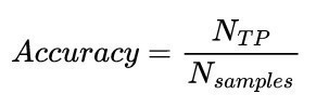
Different metrics and tools are available for the evaluation of neural networks, depending on the application. For the comparison of binary classifiers (k = 2 classes), the accuracy is specified as Accuracy. For multi-class classifiers (k > 2), the average accuracy across all classes is usually specified and also called (Average) Accuracy. It is calculated according to equation <1> . A prediction or classification is generally rated as correct (true positive) if the predicted class matches the actual class.

Fig. 9: Example of the intersection-over-union calculation

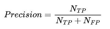
The metrics of COCO Detection Evaluation [8] are usually used to evaluate the performance (in terms of accuracy) of object detectors. The most common comparative value is the Average Precision (AP). This is an average value from average values. To calculate the value, the precision(Eq. <2>) is determined for each class at different intersection over union thresholds (IoU for short, Fig. 9). This value can also be understood as mean Average Precision (mAP). The precision describes the ratio of correctly recognized objects to the number of recognized objects. The IoU describes the overlap between the predicted object boundary and the actual object boundary.

In addition, as part of the COCO evaluation, the metrics mentioned are related to different scale levels in order to determine the performance for small, medium and large objects. These are noted as APs, APm, APl. The object area is considered in pixels.

• small  0 < area ≤ 1024
• medium  1024 < area ≤ 9216
• large  9216 < area

<1>

<2>

TP - True Positive, FP - False Positive

5 Tests and results

To check whether transfer learning and pre-trained models can be used in this application area, experiments were carried out in the field of image classification and object detection. The influence of the hyperparameters on the training behavior was mainly investigated. These are determined experimentally on the basis of standard values.

5.1 Image classification

The CNN models used here originate from PyTorch [9]. The following software versions and hardware were used during the experiments:

• Python version: 3.7.10
• PyTorch version: 1.8.1
• Torchvision version: 0.9.1
• W&B CLI Version: 0.10.32
• Graphics card: Tesla V100-SXM2-16GB (via Google Colab Pro)
• Driver version: 460.32.03
• CUDA version: 11.2

The 'Classification' data set(Tab. 3) is used to train the CNNs. From each class, 60 samples are randomly selected for the test set (N = 360), the remaining elements are used for training.

In the first experiment, 30 different network architectures from 10 families were trained and evaluated with the following standard configuration.

• Batch size 256
• Optimizer SGD
• Learn rate ^1*10-3
• Loss function Cross Entropy

In this experiment it became clear that some network architectures are better and some worse suited as fixed feature extractors. The performance of some models during training is shown in Figure 10. As can be seen, models from the family of VGGs and the AlexNet achieve an accuracy of over 95% after just 10 epochs.

Fig. 10: Accuracy progression over the training progress of different network architectures

Fig. 11: Influence of different learn rates on training using the example of ResNet-152

Fig. 12: Influence of different batch sizes on training using the example of ResNet-152

Fig. 13: Influence of the data set size

Practical tests were carried out with a number of common CNNs. These were specifically tested for their suitability as fixed feature extractors, as this requires particularly little training data. It was found that most of the models tested deliver good to very good results in this case, while others are unsuitable. The models of the VGG and DenseNet families as well as AlexNet showed the best results in this configuration. It turned out that the Learn Rate parameter has a strong influence on the training quality(Fig. 11). In contrast, the models were rather insensitive to changes in batch size(Fig. 12). The investigation of the influence of the data required for training revealed that the estimated value of 100 samples per class was more than sufficient. Already after 50 samples, no significant improvements of the model were recognizable(Fig. 13).

5.2 Object detection

In the previous section, it was shown that CNNs are well suited for classifying electronic components in radiographic images. Since the networks investigated there are often used as backbones in object detectors, it is reasonable to assume that good results can also be achieved for this application. In addition to Detectron2, the YOLOv5 PyTorch implementation [10] was also used to train the object detector. The Faster R-CNN (two-stage) and RetinaNet (one-stage) architectures from the Detectron Model Zoo [11] were used here. The influence of the batch size on the training process and the results was again investigated. It was found that reducing the batch size to 2 (0.5x starting value) or increasing it to 8 (2x starting value) has only a minor effect on the training. Table 4 is an example for the RetinaNet model.

Table 6: Influence of data set quality on object detection on unknown input data

Model	Data source	Classes	APs
YOLOv5l	internal	1	65,31
		6	62,11
	internal + external	1	66,61
		7	68,01
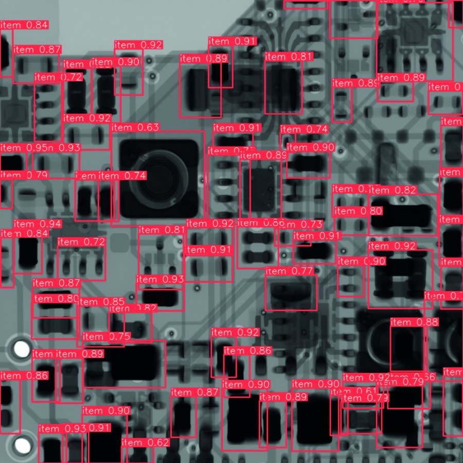
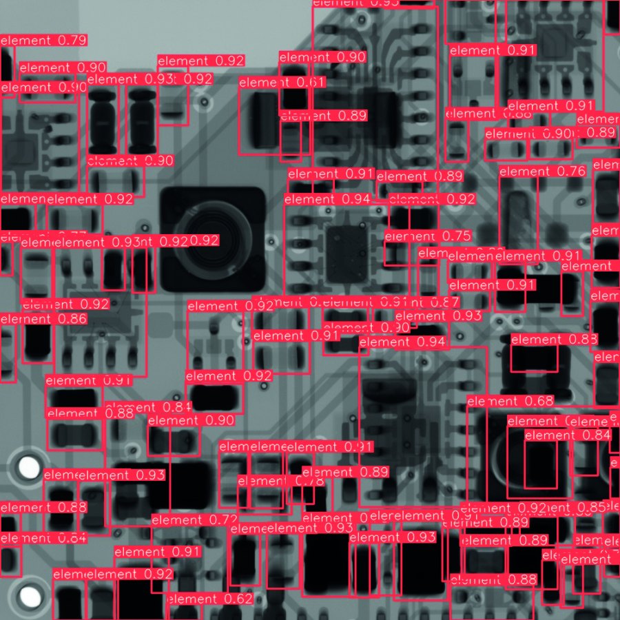
Data set detection 1 / number of classes = 1		Data set detection 2 / number of classes = 1
Objects recognized as components are highlighted with a red frame
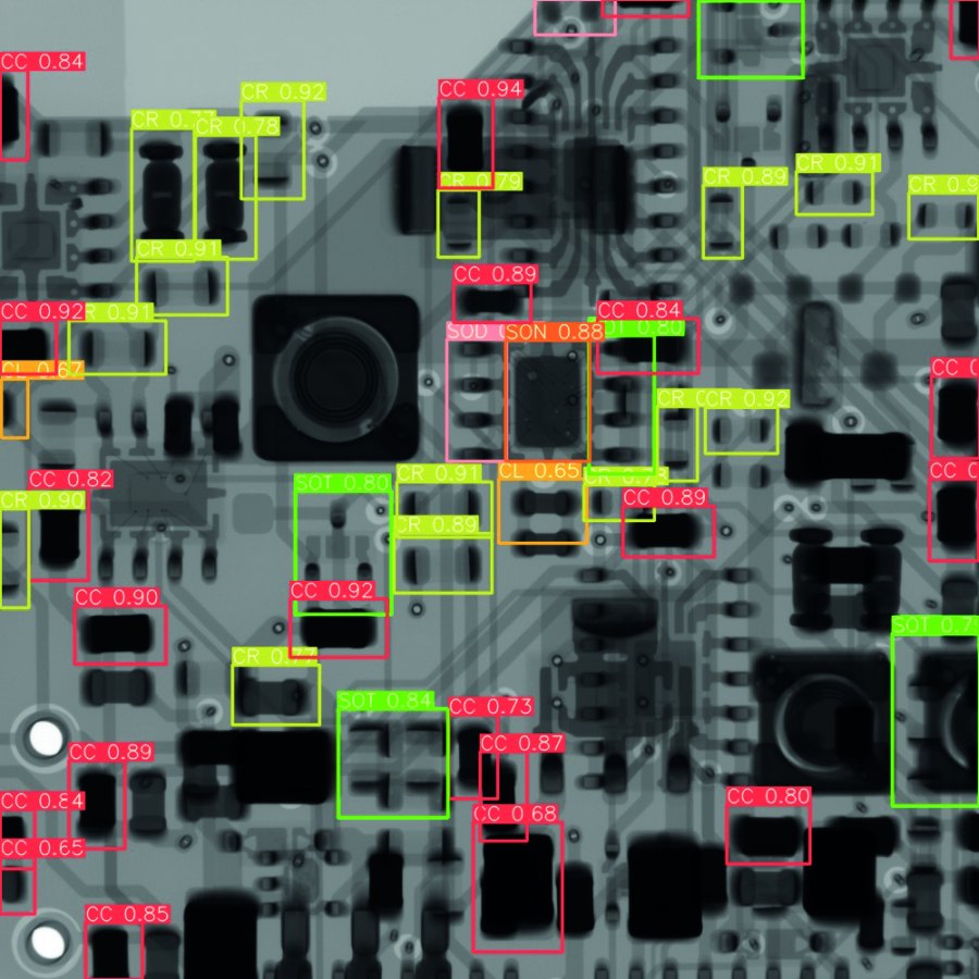
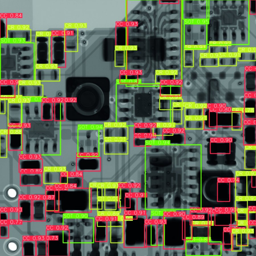
Data set detection 1 / number of classes = 6		Data set detection 3 / number of classes = 7
Detected components that can be assigned to a class with a defined probability (P ≥ 50%) are given a clear frame (CC = red, CL = dark yellow; CR =P yellow; SOT = green, SOD = pink; SON = orange)

In a further experiment, the influence of frozen layers was investigated. This refers to the number of layers that are not optimized during the training process. The default setting is to 'freeze' the first two layers. In the experiments, 3, 4, 6 and 10 layers were 'frozen'. This had a very strong influence on the accuracy, especially when detecting small and large objects (Table 5).

Investigations into the influence of the learn rate showed that increasing it generally increases the accuracy of the model.

Finally, the influence of the 'quality' of the training data sets provided on the result of object recognition on an unknown test object was to be evaluated. The following data sets were used and trained on the YOLOv5l model:

• Data set 'Detection 1' (internal), with 1 class (binary detection)
• Data set 'Detection 1' (internal) with 6 classes (multi-class detection)
• Data set 'Detection 2' (internal + external) with 1 class
• Data set 'Detection 3' (internal + external), with 7 classes

It was shown that the quality of the object detection can be improved by a higher variety and data set size. Table 6 shows the object detection results of all four variants for the same input image. This is a section of an X-ray image of a real assembly (Arduino single-board computer), which was not previously included in any of the data sets. The reliability and quantity of detections is increased in both cases after training with a combined data set.

6 Summary

It has been shown that transfer learning is a suitable method for both classification and object recognition of electronic components in radiographic images. As a rule, neural networks require a very large database in order to recognize underlying patterns and structures. The approach chosen here makes it possible to transfer the knowledge of a neural network from a source domain to a target domain. It has been shown that this can significantly reduce the data required and the time needed for training. Suitable training datasets can be generated with a manageable amount of effort, but will also increasingly be generally available. In addition, there are a large number of suitable software platforms and ready-made models that can be adapted to specific requirements even without in-depth programming knowledge. A detailed description of all the work and results achieved can be found in [12].

Literature

[6] J. Yosinski; J. Clune; Y. Bengio; H. Lipson: How transferable are features in deep neural networks?, Adv. Neural Inf. Process. Syst., vol. 4, no. January, 2014, 3320-3328
[7] D. Soekhoe; P. van der Putten; A. Plaat: On the impact of data set size in transfer learning using deep neural networks, 2016, 50-60
[8] COCO Consortium, COCO detection evaluation, COCO Common Objects in Context, 2022. https://cocodataset.org/#detection-eval
[9] Models and Pre-Trained Weights, https://pytorch.org/vision/stable/models.html
[10] ultralytics/yolov5: YOLOv5 in PyTorch, https://github.com/ultralytics/yolov5
[11] facebookresearch/detectron2: Detectron2 is FAIR's next-generation platform for object detection, segmentation and other visual recognition tasks, https://github.com/facebookresearch/detectron2
[12] J. Schmitz-Salue: System design for transfer learning of neural networks for object recognition of electronic component types in radiographic images, diploma thesis, TU Dresden 2021